On-Device Learning Note
Table of contents
- Relevant Notions
- Limitations & Directions
- On-device Adaptation
- Transfer Learning
- Federated Model Learning
- Security Concerns
- Components in an AI Framework
- Efficient Models
- Model Optimizations
Harvard Edge CS249R - Chapter 12 On-device Learning
Relevant Notions
On-Device Leaning, which is closed to TinyML, also called Federated Learning, is for embedded and edge ML deployments.
Limitations & Directions
On-device learning has limitation with i)compute resources, and ii)dataset size, accuracy, and generalization.
Comparatively, cloud learning is more complex, more efficient, and larger.
- For complexity, on-device learning might limit the number of layers & parameters.
- For efficiency, on-device learning might need quantization & pruning.
- For large-size, on-device learning might need compression.
On-device learning has challenges in small dataset size, accuracy & efficient tradeoff, and generalization. Consider the speed requirement of some tasks and the non-IID (independent & identically distributed) data that on-device learning handling.
- Susceptible to over-fitting due to small dataset.
- Low-quality noisy user-generated data is affecting accuracy.
- While one iteration time is fast, overall training time could be long.
- Size & speed & accuracy tradeoff, think of an 8-bit quantized model vs a 32-bit one.
On-device Adaptation
Some details see here - Model Optimizations.
Resource consumption comes from → so to have corresponding solutions: i)ML model itself → reduce the complexity; ii)Optimization Process → modify optimizations; iii)Storing & processing the using datasets → new storage-efficient data representations.
Reducing model complexity
Traditional ML Naive Bayes classifier, support vector machine (SVM), linear regression, logistic regression, select decision tree.
Pruning Remove neurons or connections in the network, that don’t contribute significantly to the prediction.
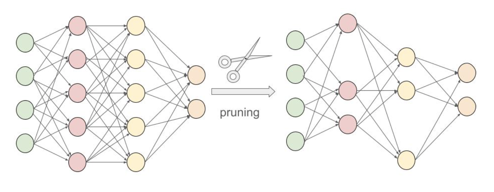
Fig 12.2 Network pruning.
Existing frameworks, to reduce memory overhead, for continuous learning (lack of lightweight, back-propagation). alibaba/MNN, apache/TVM, TensorFlow Lite.
Cutting-edge methods Quantization-aware scaling (QAS), sparse updates.
Modifying optimization process
Quantization-aware scaling
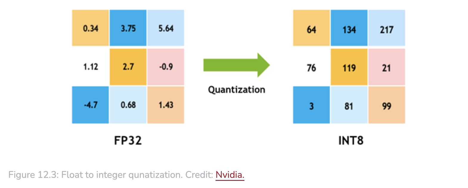
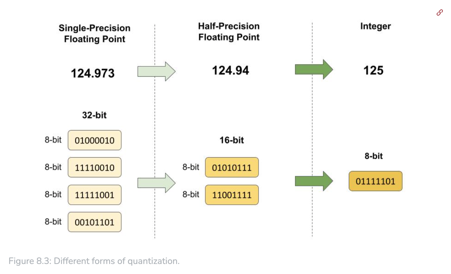
Quantization is a process of mapping a continuous range of values to a discrete set of values, including reducing precision of weights and activations from 32-bit floating point to lower-precision format eg 8-bit integers).
QAS tries to minimize the quantization error, by adjusting the scale factors during quantization, based on the distribution of weights and activations, without hyper-parameters tuning.
This involves 2 steps: i)quantization-aware training, ii)quantization & scaling.
Sparse updates
Reduce memory consumption of full backward computation, by pruning gradient during backward propagation, ie skipping computing gradients of less important layers and sub-tensors.
Contribution analysis is needed for optimizing sparse update scheme, which measures the the accuracy improvement from biases and weights.
Layer-wise training
Sequential layer-by-layer training, instead of training end-to-end, avoid having to store intermediate feature maps.
Trading computation for memory
Release some of the memory storing intermediate results, which recomputed as needed.
New data representations for data compression
Prioritize sample complexity, which is the amount of data required.
Reduce dimensionality & volume of training data, eg
i)by transforming training data into a lower-dimensional embedding & factorizing them into a dictionary matrix, multiplied by a block-sparse coefficient matrix;
ii)by representing words from a large language training dataset in a more compressed vector format.
Transfer Learning
A model developed for a particular task can be reused as the starting point for a model on a second task. Regarding the context of on-device AI, this is to fine-tune a pre-trained model using smaller dataset on the device. Knowledge transfer, so called sometimes.
Eg researchers (Esteva et al.,2017) developed a transfer learning model to detect cancer in skin images, which is pre-trained on 1.28 million images to classify a broad range of objects and then specialized for cancer detection, by training on a dermatologist-curated dataset of skin images.
Pre-deployment specialization
Workflow: start with a pre-trained model → fine-tuning → validation → deployment.
Post-deployment specialization (on-the-fly personalization)
Workflow:
data collection → model fine-tuning → validation → deployment.
Core concepts
- Source task, target task.
- Representation transfer, includes (data) instance transfer; feature-representation transfer; parameter (weights) transfer.
- Fine-tuning.
- Feature extraction, ie use pre-trained model as a fixed feature extractor.
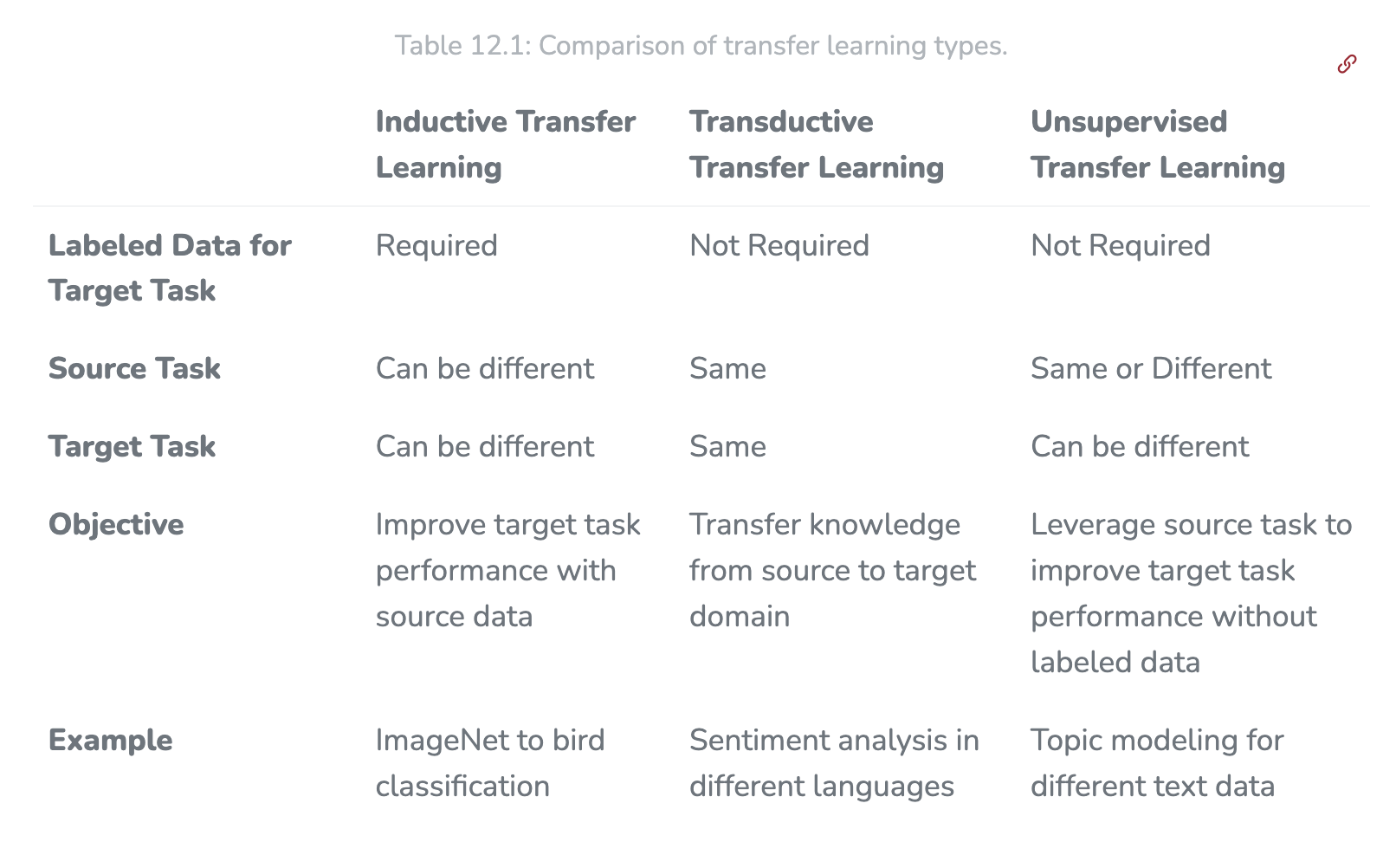
Taxonomy
Inductive transfer learning; transductive; unsupervised.
Constraints & considerations
- Domain similarity
- Task similarity
- Data quality an quantity
- Feature space overlap
- Model complexity
Federated Model Learning
A solution to train models partially on edge devices, only communicate model updates to the cloud.
FederatedAveraging
Google proposed a algorithm, FederatedAveraging, in 2016.
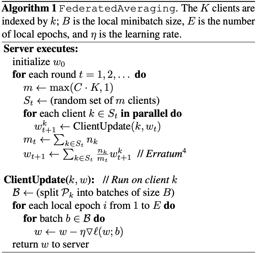
Performs SGD over several different edge devices. Figure 12.5: Google’s Proposed FederatedAverage Algorithm. Credit: McMahan et al. (2017).
Key vectors for further optimizing FL
- communication efficiency
- model compression
- selective update sharing
- optimized aggregation
- handling non-IID data
- client selection
G-Board, as an example of federated learning.
MedPerf, an open-source benchmarking for federated learning.
Security Concerns
- Data poisoning
- Adversarial attacks
- Model inversion
- On-device learning security concerns: transfer-based attacks; optimization-based attacks; query attacks with transfer priors.
- Mitigation of on-device learning risks: similarity-unpairing (diminish the similarity between on-device models and full-scale models); CleverHans tool; defense distillation.
- Securing training data: encryption; differential privacy; anomaly detection; input data validation.
- On-device training frameworks: Tiny Training Engine; Tiny Transfer Learning; Tiny Train.
Components in an AI Framework
Reference: Chapter 4 AI Workflow, and Chapter 6 AI Frameworks
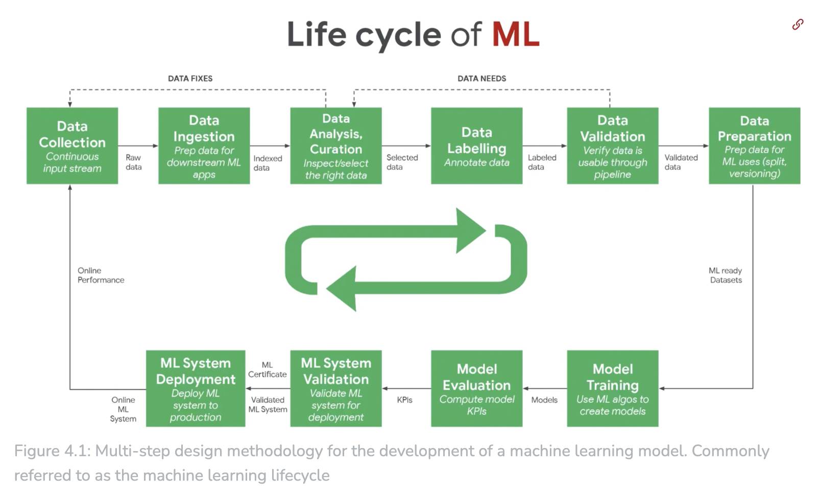
Reference: Chapter 4 AI Workflow. 4.1 Overview.
Computational Graph
There are static one, ie executed after definition, and dynamic one, ie built on-the-fly.
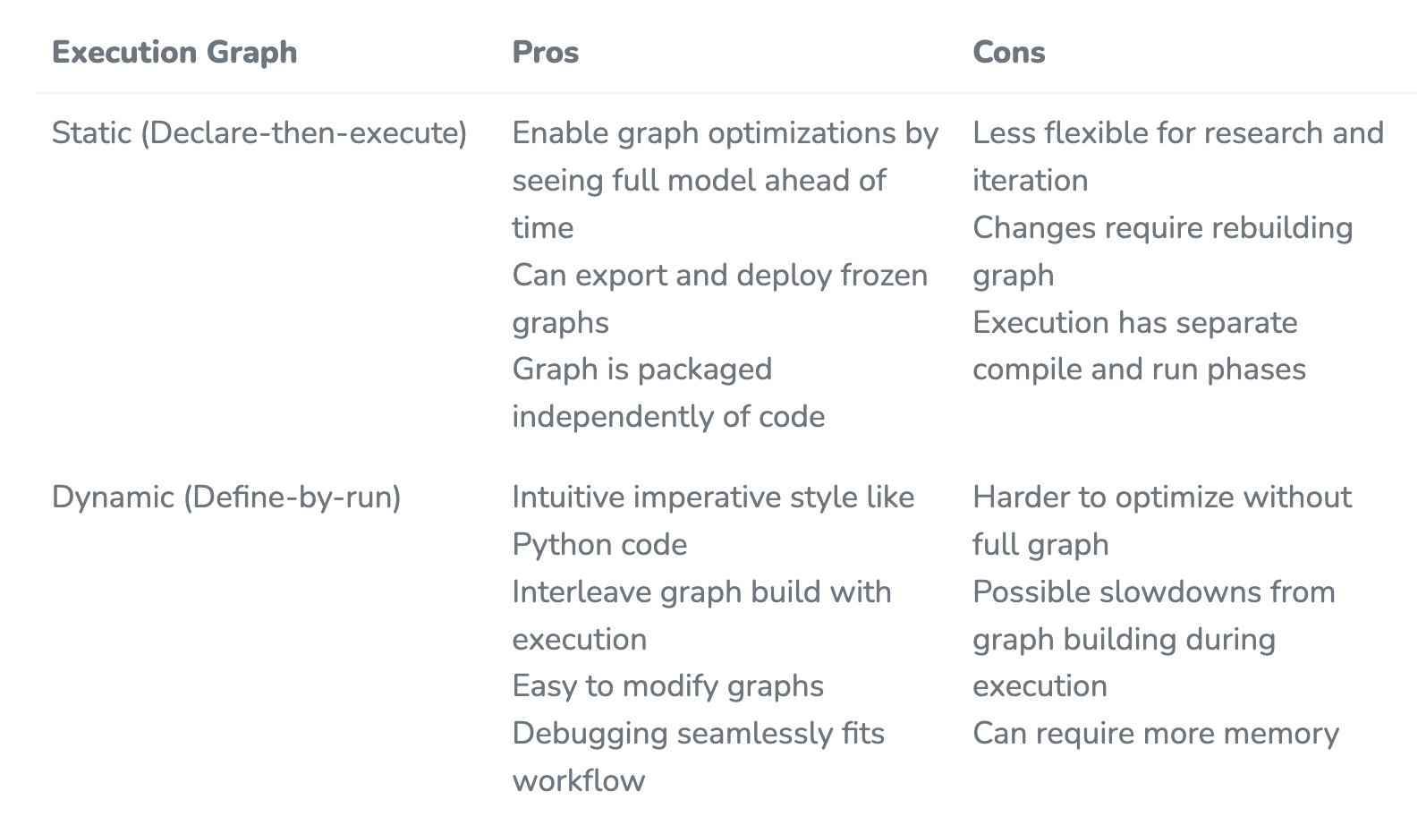
Figure in 6.4.2.
Ahead-of-Time compilation of static one results in faster execution compared with dynamic one.
Optimization advantages of static computational graphs:
- graph fusion
- constant folding
- memory layout optimization
- parallelization
- hardware-specific optimizations
ML inference frameworks for embedded systems & microcontrollers
| TensorFlow Lite Micro | Tiny Engine | CMSIS-NN |
|---|---|---|
| an interpreter | compiler-based | a software library |
Comparison of above three frameworks, see here.
Future
ML systems Breakdown:
AI applications → Computational graphs → Tensor programs → Libraries and runtimes → Hardware primitives.
High-performance compilers & libraries
Horizontal perspective.
TensorFlow XLA, CUTLASS (Nvidia), TensorRT (Nvidia).
ML for ML frameworks
Hyperparameter optimization, eg Bayesian optimization, random search, grid search.
Neural architecture search (NAS).
AutoML.
Look into AI training
Optimization on optimization algorithms
Specifically, optimizations on commonly used SGD (Stochastic gradient descent).
- Momentum, 🉑 within consistent gradient directions.
- NAG (Nesterov Accelerated Gradient).
- RMSProp, 🏅 in natural language processing.
- Adagrad, 🉑 within sparse gradient.
- Adadelta
- Adam, 🎖️ in computer vision.
Benchmarking of optimizations Evaluations would consider among training loss curves, generalization error, sensitivity to hyperparameters, computational efficiency (AlgoPerf, 2023).
Hyperparameter tuning
Before SOTA, for faster convergence and controllable gradient divergence, tuning methods are like, batch normalization through tuning aspects of internal covariate shift, adaptive learning rate, etc.
Some typical key hyperparameters across ML algorithms 🐟
- Neural networks: learning rate, batch size, number of hidden units, activation functions.
- Support vector machines: regularization strength, kernel type and parameters.
- Random forests: number of trees, tree depth.
- K-means: number of clusters.
Some prominent hyperparameter search algorithms 🌟
- Grid search
- Random search
- Bayesian optimization
- Evolutionary algorithms
- Neural architecture search
To know the tuning works from some system implications 🍥
- Lower computational costs
- Reduced training time
- Resource efficiency (Benefit from faster & stable convergence, and shorter training time.)
Some auto tuners 🧶
For big ML, Google’s Vertex AI Cloud (Vertex AutoML), a commercial auto-tuning platform.
For tiny ML, Edge Impulse’s Efficient On-device Neural Network Tuner (EON Tuner), an automated hyperparameter optimization tool designed for microcontroller ML models.
Runtime complexity of matrix multiplication
As neural networks training comprise linear transformation operation (ie matrix multiplication) and non-linear transformation (ie activation), the former one occupies most of the computing time.
Consider a layer with M-dimension input and N-dimension output, consists K-dimension neurons. The matrix multiplication (by multiply-accumulate operations) happens for computing outputs of inputs * neurons, ie a (M1) matrix * (1K) matrix, supposing batch=1 → results in O(M*K). While for element-wise activation function, it is in O(N).
To reduce the time of these linear algebra operations, some optimizations for general sparse/dense matrix-matrix, and matrix-vector operations: 🍤
- Optimized math libraries, eg cuBLAS (for GPU acceleration)
- Lower precision formats, eg FP16, INT8, with accuracy permission
- Special hardware for matrix multiplication, eg TPU (Tensor processing units)
- Sparsity-aware computations & data storage formats, for zero-flood parameters (sparsity exploitation)
- Algorithms like FFT (Fast Fourier Transforms)
- Reduce layer widths & activations in model architecture design
- Compression techniques, eg quantization, pruning, distillation
- Hardware for parallelization of computation
- Caching / pre-computing results, to reduce redundant operations
Computation vs. Memory
Computational profiles are different during process of training and inference. It is memory-bound (measured through operations/byte, memory bandwidth), vs compute-bound (measured through FLOPS, or operations/second, arithmetic throughput).
Batch size matters in the above computational profiles.
Hardware optimization is motivated by the above bottlenecks, more compute-side now than memory-side. Model architecture poses different computational or memory bottlenecks as well, eg Transformers and MLPs, vs CNNs.
Training parallelization
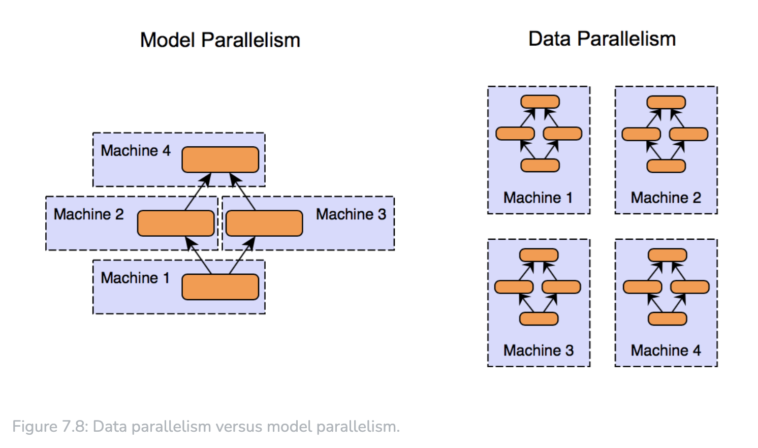
Data parallelism
This could be used both for small and big models.
Typical workflow:
Divide the dataset → replicate the model → parallel computation → gradient aggregation → parallel parameter update → synchronization.
Model parallelism
This could be used for big models.
Typical taxonomy:
- Layer-wise parallelism, ie layers on different devices.
- Filter-wise parallelism, for CNNs, ie kernels on different devices.
- Spatial parallelism, eg for images, ie regions on different devices.
Efficient Models
Make models with less parameters have strong performance.
A Perspective of architecture
- MobileNets: depth-wise separable convolutions + inverted residuals + linear bottlenecks, for mobile & embedded vision application models.
- SqueezeNets: small size by using a ‘fire module’ + delayed downsampling for a larger feature map.
- ResNet variants (Residual Networks): skipping connections / shortcuts; ’squeeze & excitation’, eg ResNet-SE; grouped convolutions, eg ResNeXt.
A Perspective of compression
- Pruning: remove certain weights or neurons from network based on specific criteria. Taxonomy: weight pruning, neuron pruning, structured pruning.
- Quantization: reduce the number of bits representing the weights & biases of the model. Use 16-bit or 8-bit to replace 32-bit.
- Knowledge distillation: train a smaller ‘student’ model to replicate the behavior of a larger ‘teacher’ model, ie transfer knowledge from large one to lightweight one.
A Perspective of hardware
Specifically, inference hardware.
- Edge TPUs: inference runs faster than on CPUs, as they are custom-build ASICs to accelerate machine learning by optimizing tensor operations, offering high throughput for low-precision arithmetic, which is designed specifically for neural network machine learning.
- NN accelerators: Fixed-function neural network accelerators. Eg standalone chips, or part of a larger SoC (system-on-chip) solution. They are optimized for specific operations, eg matrix multiplications, convolutions. Good for TinyML devices with power or thermal constraints.
A Perspective of numerics
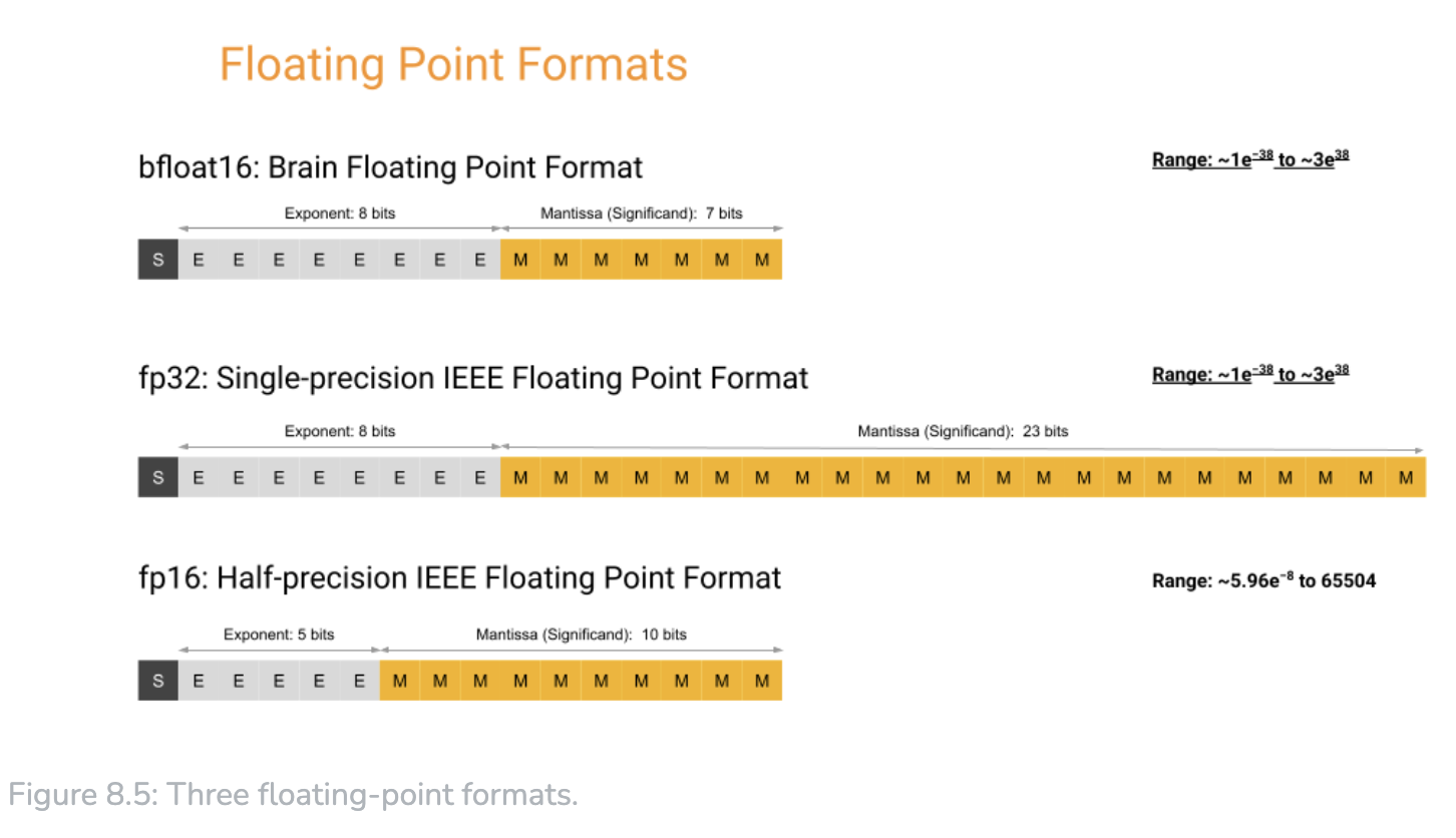
- Floating point:
- FP32, single-precision floating point, floating point 32-bit
- FP16, half-precision floating point, floating point 16-bit
- BF16, Brain Floating Point, a 16-bit numerical format
- Integer: 8, 4, 2 -bit integer representations, mainly used in inference. Eg for BNNs (Binary neural networks), where weights & activations are constrained to one of 2 values, [+1, -1].
- INT8, 8-bit integer
- INT 4-bit integer
- Variable bit widths: Low bit-width numerics.
- Binary, 1 bit per parameter
- Ternary
Considerations
- Computational efficiency
- Memory efficiency
- Power efficiency
- Noise introduction
- Hardware acceleration
Metrics
Accuracy & Efficiency tradeoff.
And metrics:
- FLOPS (Floating Point Operations per second), lower for on-device models.
- Memory usage, storage & RAM, minimal memory footprints for edge devices.
- Power consumption, lower for IoT devices.
- Inference time, aligns with real-time demands.
Some benchmark datasets mentioned for providing standardized performance metrics:
- ImageNet 2015
- COCO 2014
- Visual Wake Words 2019
- Google Speech Commands 2018
Model Optimizations
From software to hardware: efficient model representation → numerics representation → hardware implementation.
Efficient model representation
Pruning, model compression, edge-friendly model architectures.
Pruning
Remove redundant / non-essential components of the model, eg connections between neurons, neurons, layers, activations.
- Typical methods:
| structured pruning (in training or after training) Towards model-specific substructures. | i) Structures to target for pruning, eg neurons, channels or filters (in CNNs), layers. ii) Establish a criteria for pruning, use some scores as quantitative metrics, eg - weight magnitude, based on absolute values of the weights; - gradient, low magnitudes have little effect on the loss; - activation, consistently low values suggest less relevance; - Taylor expansion, approximates the change in loss function from removing a given weight. iii) Select a pruning strategy. - iterative pruning, eg remove channels results in accuracy degradation. - one-shot pruning, compress models rapidly by a targeting model size, sparsity level, available compute, acceptable accuracy losses. |
|---|---|
| unstructured pruning (after training) Towards individual weights. | More flexible than structured pruning, but challenge with sparse representations. Comparison between structure pruning and unstructured pruning, https://harvard-edge.github.io/cs249r_book/contents/optimizations/optimizations.html#tbl-pruning_methods |
| iterative pruning | |
| bayesian pruning | |
| random pruning | |
| sensitivity & movement pruning | |
| lottery ticket hypothesis | Iterate until accuracy stop significantly degrade: i) randomly initialize the weights; ii) train the network until convergence; iii) prune a percentage of the lowest weights; iv) reset weights to initial values. |
- Further reading: 2023 A Survey on Deep Neural Network Pruning: Taxonomy, Comparison, Analysis, and Recommendations.
Model compression
Knowledge distillation, low-rank matrix factorization, tensor decomposition.
| Knowledge distillation | Train a smaller student model to mimic a larger pre-trained teacher model. Basic concepts: - Use soft targets derived from teacher’s probabilistic predictions, ie a temperature-scaled softmax function with [teacher’s output] → soften probability distributions over classes. - Loss function matters for distillation loss, between teacher & student, and classification loss, between student & true labels. KL (Kullback-Leibler) divergence is commonly used. - Temperature scaling in softmax function, a parameter controls the granularity of information distilled from teacher. Higher produces softer, and more informative distributions. |
|---|---|
| LRMF (Low-rank matrix factorization) | A mathematical technique in linear algebra & matrix factorization, to approximate a given matrix, by decomposing it into two or more lower-dimensional matrices, as a product of lower-rank matrices. Cross-realm eg, in recommendation systems, the user-item interaction matrix is factorized to capture latent factors related to user preferences & item attributes. But there is tradeoff between fewer parameters to store m * k + k * n & more computations in runtime O(mkn) , where k is the rank as a challenging hyper-parameter.Also information loss during factorization need to be noted. |
| Tensor decomposition | Higher-dimensional analogue of matrix factorization. Challenges as well, information loss, and nuanced hyper-parameter tuning. |
Edge-aware model design
Design edge ML models through device-aware NAS (neural architecture search).
- Typical model design techniques:
| Depth-wise separable convolutions (commonly used in image processing) | i) depthwise convolution, each input channel is convolved independently with its own set of learnable filters. ii) pointwise convolution, combine output of depthwise convolution channels through a 1x1 convolution, creating inter-channel interactions. |
|---|---|
| An Example: SqueezeNet 2016 | |
| An Example: MobileNet 2017 | |
| An Example: EfficientNet 2023 | |
- Streamline model architecture search. Eg TinyNAS 2020, MorphNet 2018.
Efficient numerics representation
Lower-precision numerics bring tradeoff between numerical accuracy & computational efficiency. Hardware-software co-design for facilitating compatibility with edge devices.
Taxonomy: Integers; Floating-Point numbers; Variable bit widths.
A Perspective of precision: double precision (Float64); single precision (Float32); half precision (Float 16); bfloat16 (Brain Floating-Point format in 16bits); integer.
A Perspective of numeric encoding and storage, for lower precision alternatives to 32-bit floats: bfloat16; posit; Flexpoint; BF16ALT; TF32; FP8.
Nuances in consideration: memory usage; impact on model parameters & weights; computational complexity; hardware compatibility; precision and accuracy tradeoffs.
Trade-off use cases: autonomous vehicles; mobile health applications; HFT (high-frequency trading) systems; edge-based surveillance systems; scientific simulations.